Recitation 3
Homework Tips
- Be familiar with the What Can I Ask On Diderot? policy
- Talk to other students taking the course – they can help you and you can help them.
- Feel free to meet other students during the Collaboration Space – every Tuesday in GHC 4303.
- Look for the “Common Problems in Homework x” post on Diderot before asking questions online.
TA Hours
- Come this week! Don’t wait until the last week.
- Construct a minimal counter-example : a simplest test case that fails.
import numpy as np
import matplotlib.pyplot as plt
from sklearn.linear_model import LinearRegression
Linear Classification
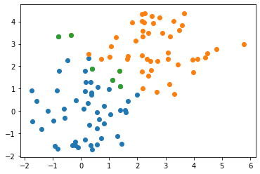
Usually we talk about linear regression: inferring a continuous value as a linear function of input variables. In this homework, we’re using linear regression to predict a category variable. Let’s see what this looks like on a simple test dataset:
n=50
data = np.concatenate((np.random.normal(size=(n, 2)), np.random.normal(size=(n, 2)) + 2.5))
cls = np.array([-1]*n + [1]*n)

plt.scatter(data[cls==-1,0], data[cls==-1,1])
plt.scatter(data[cls== 1,0], data[cls== 1,1])

We fit a simple linear regression model to this data and examine the output. Notice that the output is continuous, not discrete.
model = LinearRegression()
model.fit(data, cls)
pred = model.predict(data)

pred[:5]
Let’s draw the scatter data and highlight misclassified points:
plt.scatter(data[pred<0,0], data[pred<0,1])
plt.scatter(data[pred>0,0], data[pred>0,1])

# Plot misclassified points:
errs = ((cls==-1) & (pred>0)) | ((cls==1) & (pred<0))
plt.scatter(data[errs,0], data[errs,1])
Lets visualize the classifier using regularly-spaced points:
xx, yy = np.meshgrid(np.linspace(-3, 6, 101), np.linspace(-3, 6, 101))
grid = np.vstack([xx.ravel(), yy.ravel()]).T
ccls = model.predict(grid)
plt.scatter(grid[ccls<0,0], grid[ccls<0,1])
plt.scatter(grid[ccls>0,0], grid[ccls>0,1])

# Post the original data division as well:
plt.scatter(data[cls==-1,0], data[cls==-1,1])
plt.scatter(data[cls== 1,0], data[cls== 1,1])
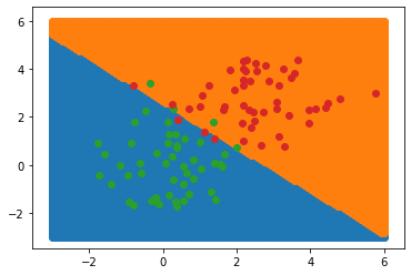
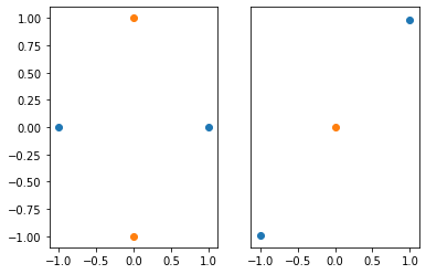
Notice that the class boundary is a line; this is characteristic of a linear classifier. We cannot separate classes like these using a linear classifier:
plt.subplot(1, 2, 1)
plt.scatter([-1, 1], [0, 0])
plt.scatter([0, 0], [-1, 1])

plt.subplot(1, 2, 2)
plt.yticks([])
plt.scatter([-1, 1], [-1, 1])
plt.scatter([0], [0])
F1 vs Accuracy
In hw3_text, we introduce the $F_1$-score to measure the performance of a binary classifier. We define this in terms of the number of true and false positives and negatives in our classifier.
| Predicted | Actual | |
|---|---|---|
| true positive | T | T |
| false positive | T | F |
| false negative | F | T |
| true negative | F | F |
To calculate the $F_1$ score, we can calculate: \(\begin{align*} \text{precision} & \gets \frac{\text{true positive}}{\text{true positive} + \text{true negative}} \\ \text{recall} & \gets \frac{\text{true positive}}{\text{true positive} + \text{false positive}} \\ F_1\text{ score} & \gets 2 \cdot \frac{\text{precision} \cdot \text{recall}}{\text{precision} + \text{recall}} \end{align*}\)
Why?
We care about this because it works when you want to measure classifier performance on rare events.
For example, lets look at a pair of ficticious medical test in a population where 1% of people have some disorder.
When Zico’s Magic Classifier (ZMC) and the much simpler Always False Classifier (AFC) are run on 1000 people, they both obtain 99% accuracy. Here are the confusion matrices for both:
| Always False Classifier | Actual True | Actual False |
|---|---|---|
| Predicted True | 0 | 0 |
| Predicted False | 10 | 990 |
| Zico’s Magic Classifier | Actual True | Actual False |
|---|---|---|
| Predicted True | 10 | 10 |
| Predicted False | 0 | 980 |
The accuracy for both classifiers is 99%, despite AFC not depending on the data (and consequently being useless). In this example, accuracy does not tell us which classifier is better.
Let’s calculate the $F_1$ score for both classifiers:
| Precision | Recall | $F_1$ score | |
|---|---|---|---|
| ATC | $\frac{0}{0}$ | $\frac{0}{10}$ | $0$ or NaN |
| ZMC | $\frac{10}{20}$ | $\frac{10}{10}$ | $\frac{2}{3}$ |
The $F_1$ score is good when you want measure your classifier’s performance on catching rare events.